Biacore X100 reference portal

Follow the steps below in the order given when evaluating kinetic data:

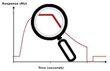
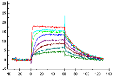
1. Inspect the sensorgrams visually

• Check each sensorgram for general shape and appearance.
• If any of the sensorgrams have major disturbances (e.g. injection of air, excessive noise, unstable baseline etc), exclude these from the data set to be analysed.
• Transient disturbances such as spikes from air bubbles can be deleted from the sensorgrams at the evaluation stage.
• Transient shifts at the beginning and end of the sample injections are a common artefact of reference subtraction, resulting from slight errors in sensorgram alignment. These can be excluded from the data used for fitting and do not need to be removed from the sensorgrams.
• Check replicate sensorgrams for similarity. If replicates are significantly different, kinetic constants extracted from the data will not be reliable.

2. Fit the data to an interaction model

Choose the simplest interaction model that is consistent with your experimental system. Choose 1:1 interaction unless you have good reason to do otherwise

Global versus local fitting

Use the global fitting function whenever possible. Global fitting finds the best fit to all of the sensorgrams simultaneously, in contrast to local fitting which fits to only one sensorgram at a time. Selected parameters such as rate and affinity constants are constrained to have a single value for all sensorgrams in the data set.

Global fitting to the entire set of experimental data is mathematically more robust than local fitting to single sensorgrams. Local fitting can give more exactly fitted curves, but can hide discrepancies between the curves.

Sensorgram subtraction for kinetic measurements

Use on-line reference subtraction in Biacore system where this is supported. On systems, which do not support on-line reference subtraction, run parallel analyses on a reference surface and subtract the reference from the sample in the evaluation software.

Always include zero-concentration samples in the assay. Subtract zero-concentration sensorgrams from the other sensorgrams in the series. This operation eliminates any systematic variations in the sensorgrams that are not removed by reference subtraction, and can significantly improve the robustness of the subsequent curve fitting. The procedure of first subtracting the reference response and then subtracting the zero-concentration sensorgram is termed double-referencing, and is strongly recommended for analyses where the response levels are close to the detection limit of the system.

Since zero-concentration samples do not contain analyte, the sensorgrams for zero-concentration samples belonging to different compounds should in principle be interchangeable, provided that all compound samples are prepared in the same buffer and in the same way.

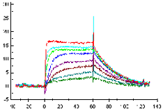
3. Inspect the fit

There are several numerical and graphical aids to judge how well the chosen model fits the experimental data. However, with a little practice, visual inspection of the fitted curves overlaid on the sensorgrams is often the best way to judge the results. Residual plots showing the difference between experimental and calculated data can be helpful.

In general, residual values will be larger for global fitting to all curves simultaneously than for local fitting to each curve individually. This is because global fitting constrains certain parameters to have the same value for all curves.

In an excellent fit, the fitted curves correspond closely to the sensorgrams over the whole range. The model is a fully acceptable description of the experimental data. Excellent fits are rare unless a major effort has been made in sample preparation and experimental execution.

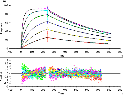
Example of a good fit

In a good fit, the fitted curves correspond reasonably well to the sensorgrams. There may be minor discrepancies in the response levels reached or in the shapes of the curves, but these are small in relation to the overall response levels. Whether the fit is acceptable or not must be judged in relation to the purpose of the experiment. Experimental variations and unavoidable deviations from ideal behaviour in biological systems often mean that a fairly good fit is the best that can be obtained.

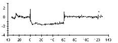
Visual inspection of the residual plot or of the fitted curves overlaid on the experimental data gives an indication of the closeness of fit. Ideally, the residuals will scatter randomly around zero over a range that corresponds to the short-term noise in the detection system. Deviations from ideal fitting appear as systematic variations in the residuals, imparting a non-linear shape to the residual plot. Judge the residual range and shape in proportion to the response ranges in the experimental sensorgrams and in relation the goal of the investigation.

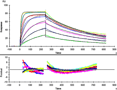
Example of a poor fit

In a poor fit, the fitted curves deviate markedly from the sensorgrams, in the response levels reached and/or the shape of the curves. In particular, fitted curves that show systematic deviations in shape from the experimental sensorgrams usually indicate that the chosen model is not suitable. Reliable kinetic constants cannot be obtained if the fit is poor.

Statistical indicators

Some statistical information provided with the results can help you to judge the fit (all parameters may not be available in all systems):

• Chi2 (χ2) is a measure of the average deviation of the experimental data from the fitted curve. Lower Chi2 values indicate a better fit. The acceptable level for Chi2 must be assessed in relation to the measured binding levels.
  The Chi2 value in an ideal situation will be approximate to the square of the short-term noise level. It is however difficult to recommend absolute values for acceptance limits for Chi2: the values need to be considered from case to case in combination with assessment of the shape of the residuals (Chi2 is related to the overall range of the residuals but is not affected by the shape of the residual curve).

• Standard error is a measure of the confidence in the reported value for the parameter. A small standard error indicates that changes in the parameter's value have a significant effect on the fitting: in other words, confidence in the value is high.
• T-values are obtained by dividing the parameter's value by the standard error, and thus provide a kind of normalised inverse standard error value. High T-values (typically above 10) indicate confidence in the parameter's value.
• U-value is uniqueness value for the kinetic rate constants. Lower values indicate greater confidence in the results.

4. Assess the results

Inspect the numerical results for reasonableness. It is sometimes possible to obtain a good fit to experimental data with values that are experimentally unrealistic.

Bulk response (RI)

For reference-subtracted sensorgrams, the bulk response values should be low (typically less than a few RU).

Analyte binding capacity (Rmax)

The theoretical analyte binding capacity can be estimated from the amount of ligand on the surface and the relative sizes of ligand and analyte. If the reported value for Rmax is unreasonably high, this may indicate non-specific binding or aggregation of analyte on the surface. If the value is unreasonably low, this may indicate loss of ligand activity.

Rate constants (k_a and k_d)

Reasonable values for rate constants for most biological interactions are:

• Association rate constant k_a :10⁴ - 10⁹ M^-1 s^-1 (measurable 10³ - about 10⁸)
• Dissociation rate constant k_d :10^-5 - 1 s ^-1 (measurable 10^-5- 10^-1)
• Mass transport constant k_t :10⁸ - 10⁹ s^-1

If reported values lie significantly outside these ranges, check the standard error or T-value for the constants. If confidence in the value is low, the evaluation procedure may generate meaningless values.

Fitting procedure

Kinetic rate constants are extracted from experimental data by an iterative process that finds the best fit for a set of equations describing the interaction. The equations are created automatically from the definition of the interaction model. The fitting process begins with initial values for the parameters in the equation set, and optimizes the parameter values according to an algorithm that minimizes the Chi2 value for the fitting. Chi2 is a measure of the average squared residual (the difference between the experimental data and the fitted curve):

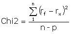
where r_f is the fitted value at a given point
r_x is the experimental value at the same point
n is the number of data points
and p is the number of fitted parameters

For sensorgram data, the number of data points is very much larger than the number of fitted parameters in the model, so

and Chi2 reduces to the average squared residual per data point. If the model fits the experimental data precisely, Chi2 represents the mean square of the signal noise.

In some situations, the fitting algorithm may be unable to find a fit for the experimental data with the initial parameter values as specified in the model. This may happen typically if the concentration unit is incorrect: for example if the unit is set to mM instead of nM in the keyword table. On occasion, however, if can be necessary to adjust the starting values for fitting parameters.

Parameters in the fitting equations

Parameters in the fitting equations are treated as either local or global variables or constants:

• Local parameters are assigned an independent value for each curve in the data set. Typical local parameters are concentration (which is different for different curves) and bulk refractive index contribution (which may be expected to vary between curves).
• Global parameters have one single value that applies to the whole data set. Typical global parameters are the rate constants for the interaction, which should in principle have the same value for all curves in the data set.
• Constants have a fixed value that is not changed in the fitting procedure. An example is the analyte concentration. Constants may also be local (separate values for each curve) or global (one value for the whole data set).

Evaluating kinetics or affinity with global rate constants gives a more robust value for the rate constants, although the curves may fit the experimental data more closely if all parameters are fitted locally. This is because local fitting allows variation between the constants obtained from different curves: when the constants are fitted globally, this variation appears in the closeness of fit rather than the reported values.

In general, kinetic constants should be fitted as global parameters and bulk refractive index contribution as a local parameter. The analyte binding capacity of the surface R_max is a global parameter and assumes that the ligand activity is unchanged between cycles in the assay): it is however justified to use a local R_max if there is reason to believe that the ligand activity may vary between cycles (e.g. in a capture assay, if the capture level varies between cycles).

Initial values

Initial values are the starting value for rate constants used in the fitting algorithm. Change these values by 2 or 3 orders of magnitude in either direction if the algorithm is clearly unable to fit the experimental data. Smaller changes in these values seldom have any effect.

Offset during injection

Offset during injection (RI) represents the bulk refractive index contribution during the injection. Ideally, the value should be zero since the sensorgrams are reference-subtracted and corrected for zero-concentration samples. The default setting of Local allows any remaining bulk effects to be eliminated by the fitting algorithm.

In some cases, rapid association and dissociation can be spuriously interpreted as bulk response in the fitting procedure. Set the parameter to Constant=0 if the values reported for RI are unexpectedly high.

Mass transfer parameters

Kinetic models include a term for mass transfer of analyte to the surface. If transport is slow compared with binding of analyte to the ligand, the transport process will limit the observed binding rate, at least partially. All models take account of this potential limitation and can extract rate constants from the data provided that mass transfer is not totally limiting.

The rate of mass transfer of analyte to the surface under the conditions of non-turbulent laminar flow that prevail in the Biacore flow cell is characterized by the mass transfer coefficient k_m (units m×s^-1):

where  D is the diffusion coefficient of the analyte
            f is the volume flow rate of solution through the flow cell
            h, w, l are the flow cell dimensions (height, width, length)

One form used in fitting models is referred to as the mass transfer constant k_t (units RU× M^-1×m×s^-1), obtained by adjusting the mass transfer coefficient approximately for the molecular weight of the analyte and for the conversion of surface concentration to RU:

A further modification of this expression gives the flow rate-independent component of the mass transfer constant (units RU×M^-1s-^2/3m^-1/3), referred to as tc in the models:

This is the simplest model for kinetic evaluation, and is recommended for first evaluation attempts unless there is good experimental reason to choose a different model. The model describes a 1:1 interaction at the surface:

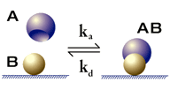
Kinetic parameters are:

k_a - association rate constant for formation of AB
k_d - dissociation rate constant for complex AB

This model is sometimes referred to as the Langmuir model, because it corresponds to the Langmuir isotherm for adsorption of substances to solid surfaces.

Transport of analyte from bulk solution to the surface is directly proportional to the bulk analyte concentration, where the proportionality constant is the mass transport coefficient which is a function of the flow rate, flow cell dimensions and diffusion properties of the analyte. This constant has units of RU∙M^-1s^-1. For globular proteins with molecular weight of the order or 50,000 daltons, typical values for the mass transport coefficient are of the order of 108 RU∙M^-1s^-1. Reported values that differ greatly in order of magnitude (e.g. 10¹² or 10¹⁴) may indicate that the parameter is not significant for the fitting (i.e. that the observed binding is not limited by mass transport).

A term for the rate of transfer of analyte from bulk solution to the surface is included in the 1:1 binding model (available as a separate model in the BIAevaluation software):

This model accounts for the presence of two ligand species that bind analyte independently of each other. The species may be different molecules or different binding sites on the same ligand molecule.

Kinetic parameters are:

k_a1 - association rate constant for formation of AB1
k_a2 - association rate constant for formation of AB2
k_d1 - dissociation rate constant for complex AB1
k_d2 - dissociation rate constant for complex AB2 

The complexity of the mathematical model limits the number of ligand species to two.

The heterogeneous analyte model is intended primarily for the situation where two analytes of different size are deliberately mixed. The model describes this competitive situation and returns two sets of rate constants, one for each reaction.

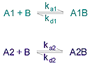
Kinetic parameters are:

k_a1 -association rate constant for formation of A1B
k_a2 - association rate constant for formation of A2B
k_d1 - dissociation rate constant for complex A1B
k_d2 - dissociation rate constant for complex A2B

The heterogeneous analyte model may be useful for determining kinetics of a small analyte indirectly by competition with a larger one. Response contributions from both analytes are taken into account, although the high molecular weight analyte is responsible for the dominant component in the observed sensorgrams.

Concentrations and molecular weights are required for both analytes. If absolute molecular weights are not known, relative values can be entered without affecting the outcome of the fitting. The model cannot evaluate interactions where the proportions and relative sizes of the analytes are unknown.

This model describes the binding of a bivalent analyte to immobilized ligand, where one analyte molecule can bind to one or two ligand molecules. The two analyte sites are assumed to be equivalent. The model may be relevant to studies among others with signaling molecules binding to immobilized cell surface receptors (where dimerization of the receptor is common) and to studies using intact antibodies binding to immobilized antigen. As a result of binding of one analyte molecule to two ligand sites, the overall binding is strengthened compared with 1:1 binding. This effect is often referred to as avidity.

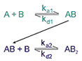
Kinetic parameters are:

k_a1 - association rate constant for formation of AB
k_a2 - association rate constant for formation of AB₂
k_d1 - dissociation rate constant for complex AB
k_d2 - dissociation rate constant for complex AB₂

Note that binding at the second site does not change the mass on the surface and therefore does not give rise to a response. For this reason, the association rate constant for the second interaction is reported in units of RU^-1s^-1, and can only be obtained in M^-1s^-1 if a conversion factor between RU and M is available. Similarly, a value for the overall affinity or avidity constant is not reported.

The general recommendation, however, is to try to immobilize the bivalent interactant and thereby avoid complications caused by the combined affinity resulting from multivalent binding (avidity). In some cases, avidity effects can be reduced by using very low ligand levels and high analyte concentrations. Low ligand levels give sparsely distributed ligand with less chance of two ligand molecules being within reach of a single analyte. High analyte concentration competes out second site binding and therefore favors formation of 1:1 complexes.